Inside Netflix’s Distributed Service Map Pipeline

By Parth Jain, Rakesh Sukumar, Yingwu Zhao, Renzo Sanchez-Silva & Nathan Fisher
A deep dive into the engineering challenges of constructing a real-time service dependency map at Netflix scale: from streaming architectures and distributed aggregation pipelines to time-travel queries and the methodology that made it work.

Introduction

In our first submit, we launched the issue: engineers at Netflix wanted a unified, real-time view of service dependencies to troubleshoot sooner, perceive blast radius, and navigate our distributed structure. We described our multi-source strategy, combining eBPF community flows, IPC metrics, and distributed tracing into bodily separate graph layers that may be queried independently or merged right into a complete view.

That submit defined what we constructed and why. This submit is about how, the engineering actuality of constructing this method at Netflix scale.

Right here’s the reality: the primary model labored completely… in our native setting. Manufacturing was a distinct story. Kafka customers fell behind. Cases ran out of reminiscence. Some nodes obtained 100x the site visitors of others. Rubbish assortment pauses consumed extra CPU than precise enterprise logic.

What you’ll be taught on this submit isn’t a hit story, it’s a studying journey. We’ll stroll by the structure selections that enabled scale, the manufacturing challenges that examined these selections, the optimization methodology that guided us by, and the teachings that apply to any distributed system. Alongside the best way, we’ll share the improvements that made it potential to course of thousands and thousands of circulation data per second, reconstruct topology at any cut-off date, and supply sub-second question responses, all whereas sustaining close to real-time freshness.

Structure Deep-Dive: Constructing for Streaming and Scale

Streaming-First: Why Actual-Time Issues

Conventional service topology methods use batch processing, aggregating information hourly or every day, then storing full snapshots. This strategy works at a modest scale however has a basic downside: by the point you see the information, it’s already previous. Throughout a manufacturing incident at 3am, an hour-old dependency map is archaeology, not observability.

Our key architectural resolution was to construct streaming-first. As an alternative of batch jobs that course of historic information, we constantly ingest circulation data from multi-region Kafka streams and IPC metrics as Server-Despatched Occasions, course of them by reactive pipelines with backpressure dealing with, and supply close to real-time topology updates, usually inside tens of minutes, in comparison with the hours-old or day-old information that batch processing approaches present.

This wasn’t nearly freshness, it was important for our use instances. Dwell occasions can’t look forward to the following hourly batch. Incident response wants present information. Change validation requires seeing fast impression. The structure needed to help steady updates whereas dealing with large scale with out falling behind.

How Backpressure Allows Actual-Time Processing
The streaming strategy created new challenges, but additionally required fixing a basic downside: how do you course of thousands and thousands of circulation data per second in real-time with out shedding information when downstream methods decelerate?

Conventional approaches fall quick at our scale:

• Unbounded queues: Easy however harmful. Hold buffering till you run out of reminiscence, then the occasion crashes.
• Drop-based circulation management: Discard information when buffers fill. Quick, however now your topology is incomplete, you’ve misplaced connection data.
• Batch processing: Course of every part, however hours later. By then, the incident is over (or worse, nonetheless taking place with stale information).

We wanted one thing totally different: the flexibility to decelerate gracefully below load with out shedding information. That is the place reactive streams with backpressure grew to become important.

Right here’s the way it works: when Stage 3 can’t write to the graph database quick sufficient, it alerts Stage 2 to decelerate. Stage 2 alerts Stage 1. Stage 1 alerts the Kafka shopper to pause. The info waits in Kafka till downstream capability returns.

Press enter or click on to view picture in full dimension

Backpressure propagates naturally by your complete system. When any stage turns into overwhelmed from site visitors spikes, GC pauses, or exterior slowdowns, the pipeline mechanically slows to a sustainable charge. No information is misplaced typically, no situations crash, the system degrades gracefully.

That is what permits “real-time” at our scale. Throughout regular operation, we course of with minimal latency. Throughout load spikes or short-term slowdowns, we decelerate slightly than fall over. The info nonetheless will get processed, just some seconds or minutes later as an alternative of instantly. For topology updates, this trade-off is appropriate: barely delayed real-time updates are vastly higher than hour-old batch information or incomplete topology from dropped data.

The price of this strategy is complexity. Reactive streams are more durable to motive about in comparison with conventional synchronous blocking fashions (we’ll focus on this extra within the challenges part). However at Netflix scale, backpressure isn’t optionally available, it’s the mechanism that retains the system working reliably below manufacturing load.

Multi-Layer Structure: Bodily Separation for Impartial Optimization

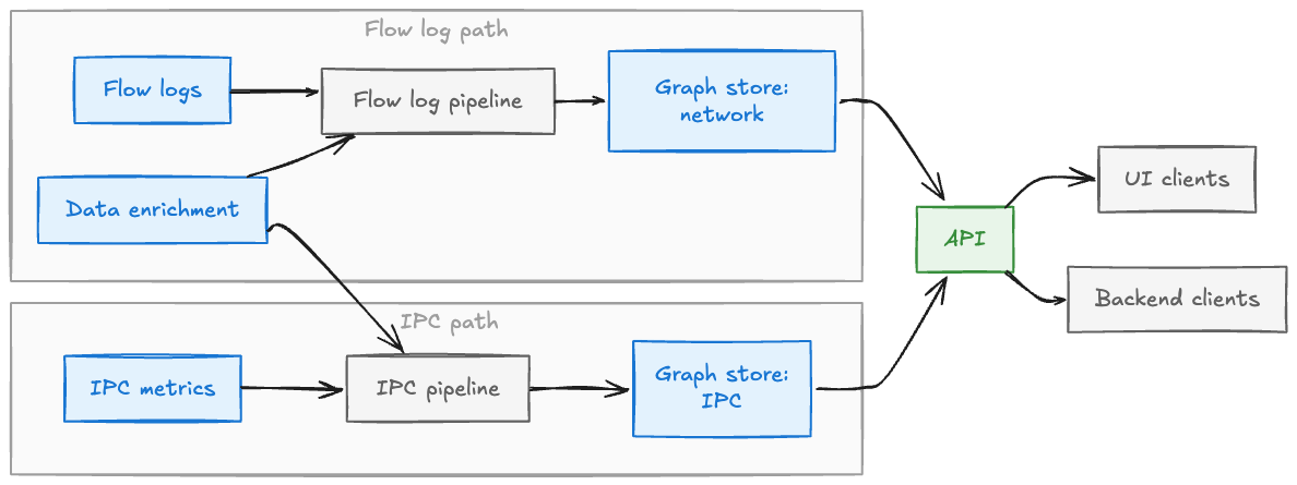
As we coated in our first submit, our multi-source strategy makes use of three bodily separate topology layers with totally different storage optimized for every:

• Community Layer: eBPF circulation logs in graph database partition, complete protection however lacks utility context
• IPC Layer: Utility metrics in a distinct graph database remoted from the one for Community Layer, wealthy endpoint particulars however solely instrumented companies
• Tracing Layer: Distributed traces in columnar storage (Parquet), precise request paths however sampled.(We cowl the tracing layer and its integration in our subsequent submit).

Press enter or click on to view picture in full dimension

Bodily storage isolation permits impartial optimization, every layer has totally different throughput, question patterns, and evolution timelines. At question time, we execute parallel queries throughout related storage methods and merge outcomes, offering unified views with sub-second latency whereas sustaining flexibility to evolve every layer independently.

The Three-Stage Distributed Aggregation Pipeline

The center of the community layer ingestion is a three-stage distributed pipeline. This structure solves a basic problem with community circulation logs: they solely present particular person community hops, not the true application-level connections we have to construct a helpful topology.

The Core Drawback: Community Intermediaries

In cloud environments, site visitors between functions not often flows instantly, it traverses intermediate community parts like load balancers, NAT gateways, API gateways, and proxies. Community circulation logs present particular person hops: App A → Load Balancer and Load Balancer → App B seem as separate flows. However what engineers want is the logical dependency: App A → App B. With out resolving these intermediaries, our topology can be cluttered with infrastructure parts slightly than displaying the service-to-service relationships that matter for troubleshooting.

The three-stage pipeline solves this:

Press enter or click on to view picture in full dimension

Stage 1: Preliminary Aggregation (FlowLog Ingestion Service)

Multi-Area Kafka (4 areas)
→ Filter invalid circulation logs
→ 5-minute time-window batching
→ Create preliminary aggregators per window
→ Distribute by way of constant hashing
→ Stream to Stage 2 by way of SSE

Stage 1 consumes circulation logs from multi-region Kafka, filters invalid data, batches them into 5-minute time home windows, and creates preliminary aggregator objects. At this stage, we’re nonetheless working with uncooked community hops, figuring out which flows contain intermediaries however not but resolving them. Aggregators stream to Stage 2 for decision.

Stage 2: Community Middleman Decision Layer (Intermediate GraphEntity Ingestion Service)

Stage 1 Aggregators (by way of SSE streams)
→ Group flows by middleman (load balancer, NAT gateway, proxy, and many others.)
→ Determine pairs: (Supply → Middleman) + (Middleman → Vacation spot)
→ Resolve to direct edges: Supply → Vacation spot
→ Observe which intermediaries have been traversed
→ Mixture metrics throughout each hops
→ Re-distribute by way of constant hashing
→ Stream to Stage 3 by way of SSE

That is the important thing step. Stage 2 performs graph decision:

1. Acquire flows by middleman: Group aggregators the place an middleman is both supply or vacation spot, creating maps of flows going TO intermediaries (Supply → Middleman) and FROM intermediaries (Middleman → Vacation spot)
2. Resolve direct edges: For every middleman, be a part of its incoming and outgoing flows to create direct utility edges (App A → App B), combining metrics from each hops
3. Outcome: Clear application-level topology displaying App A → App B as an alternative of App A → Load Balancer → App B

This decision occurs at aggregation time, not question time, with resolved edges flowing to Stage 3.

Why can’t we do that in a single stage? The basic concern is information locality. To resolve App A → Load Balancer → App B into App A → App B, we want each flows on the identical occasion to carry out the be a part of. However in Stage 1, flows are scattered throughout situations based mostly on Kafka’s partitioning. Stage 2’s vital operate is to redistribute aggregators by middleman identifier, all flows involving “Load Balancer X” path to the identical occasion for decision. That is the traditional map-reduce sample: Stage 1 maps, Stage 2 shuffles and reduces by middleman, Stage 3 performs remaining aggregation.

Press enter or click on to view picture in full dimension

Stage 3: Last Aggregation and Enrichment (GraphEntity Ingestion Service)

Stage 2 Aggregators (by way of SSE streams)Move
→ Last aggregation throughout time home windows
→ Enrich with exterior information (question key-value shops)
→ Convert to graph entities
→ Persist to graph database (throttled writes)

Stage 3 performs remaining aggregation of resolved edges, enriches graph nodes with exterior information sources (utility well being, possession, metadata), converts aggregators to concrete graph entities (nodes and edges with all properties populated), and persists them to the distributed graph database with managed throttling to respect storage system limits.

Why Three Levels, Not Two?

We initially used two phases: mixture in Stage 1, resolve and persist in Stage 2. This labored in testing however failed at manufacturing scale, Stage 2 grew to become overwhelmed by information focus.

The issue: middleman decision requires amassing ALL flows involving an middleman on the identical occasion.Consequently, the situations dealing with circulation logs for standard functions and their intermediaries grew to become ‘scorching nodes’ because of important information concentrationCompounding this, information enrichment (querying exterior shops for well being and metadata) meant the busiest situations have been additionally doing probably the most I/O.

The answer: break up duties into three phases. Stage 2 focuses purely on decision and redistributes. Stage 3 handles enrichment and persistence. This graduated redistribution (distribute, resolve, distribute once more), persist, spreads load throughout a number of situations and isolates compute-heavy decision from I/O-heavy enrichment. Even when intermediaries see 100x typical site visitors, no single occasion turns into a bottleneck.

Why Server-Despatched Occasions As an alternative of gRPC or Message Queues?

We initially used gRPC however it grew to become a efficiency bottleneck, serialization overhead, connection pool administration, and reminiscence stress for streaming responses consumed extra CPU than enterprise logic. Message queues added infrastructure complexity with out profit for our use case.

SSE proved superb: light-weight HTTP-based protocol with minimal serialization, pure backpressure integration with reactive streams, and easier connection mannequin. The lesson: business greatest practices like “use gRPC for service communication” don’t apply universally. For streaming giant volumes of pre-aggregated information, lighter-weight options could also be extra acceptable. Measure, don’t assume.

Why IPC Doesn’t Want Three Levels

Press enter or click on to view picture in full dimension

The IPC layer makes use of single-stage aggregation as a result of: (1) IPC metrics are already at utility degree, no intermediaries to resolve, and (2) information is partitioned accurately from the beginning — every node receives all IPC metrics for its assigned functions by way of constant hashing, eliminating the necessity for redistribution. This highlights a key precept: information partitioning technique determines processing structure. When information arrives with the correct partitioning, you may mixture instantly; when it doesn’t (like community flows requiring middleman decision), you want shuffle/redistribution phases.

Dynamic Load Distribution: How Hashing Works with Auto-Scaling

How can we determine which occasion receives which aggregator when our Auto Scaling Teams dynamically add or take away situations? Conventional approaches assume static clusters requiring express rebalancing, coordination companies, or handbook information motion when cluster dimension adjustments.

Our Method: Dynamic Constant Hashing

We use constant hashing with dynamic occasion discovery from our service registry. Every occasion queries the registry to get the present listing of wholesome ASG situations, maintains them in sorted order (guaranteeing all situations have the identical view), and makes use of this listing for the hash operate findOwnerInstance(aggregator.primaryKey). When ASG scales up or down, the hash operate naturally redistributes aggregators based mostly on the up to date occasion listing, no express coordination wanted.

The important thing perception: leverage current infrastructure. Our service registry already tracks ASG membership for well being checking. Utilizing it as our supply of reality offers us dynamic cluster membership without spending a dime. Constant hashing gives secure partitioning (most aggregators keep on the identical occasion throughout membership adjustments), whereas the sorted listing ensures consistency.

The Outcome

Load follows infrastructure mechanically. Throughout site visitors spikes or stay occasions, new situations instantly obtain their share. Throughout deployments, aggregators seamlessly shift to wholesome situations. This sample proved essential for manufacturing stability, no handbook intervention, no coordination protocol, simply automated rebalancing.

The V1 Journey: Main Challenges at Manufacturing Scale

Getting the preliminary model (V1) to manufacturing taught us that scale adjustments every part. What works in growth breaks in manufacturing. Each assumption will get examined. And fixing one bottleneck reveals the following.

Problem 1: Kafka Client Lag

The Drawback: Our multi-region Kafka customers began falling behind. Client lag grew from seconds to minutes, then hours. Move logs have been arriving sooner than we may course of them. If this continued, we’d by no means catch up, and our “real-time” topology would turn into more and more stale.

Investigation: We instrumented Kafka shopper metrics closely. Key findings:

• Kafka had fewer partitions than optimum for our shopper group dimension
• Every fetch operation retrieved comparatively few data
• Community socket buffers weren’t right-sized for our throughput
• Cross-region learn latency added overhead

Options Utilized:

1. Elevated Kafka partitions: Extra partitions enabled extra parallel customers in our shopper group, distributing load throughout extra situations.
2. Tuned fetch parameters: Elevated data per fetch operation, lowering the variety of community round-trips. This trades off per-message latency (we fetch bigger batches) for throughput (extra data processed per second).
3. Elevated socket obtain buffer dimension: Ensured community buffers by no means restricted fetch operations. At our scale, default buffer sizes have been too small.

Outcomes: Throughput improved considerably, and lag diminished to acceptable ranges, usually below a minute even throughout peak site visitors.

Lesson: At scale, you may’t optimize in isolation. Fixing Kafka lag revealed the following bottleneck: our situations themselves couldn’t sustain with the upper ingest charge. The pipeline moved sooner, which uncovered downstream capability issues.

Problem 2: Scorching Nodes and Knowledge Amplification

The Drawback: This was probably the most extreme manufacturing concern we confronted. Some situations in our Auto Scaling Group have been receiving 100x extra site visitors than others. Reminiscence utilization spiked. Rubbish assortment pauses grew to become frequent and lengthy. Extra CPU time was spent in GC than in enterprise logic. Finally, scorching situations would go DOWN, triggering cascading failures as their load redistributed to different situations.

Root Trigger Investigation:
Move logs for standard companies dominate site visitors quantity. A service like our authentication layer or suggestion API is known as by tons of of different companies, producing orders of magnitude extra circulation data than typical companies.

Our preliminary structure used constant hashing to find out which occasion owned aggregation for every vacation spot service. All circulation logs for a given vacation spot are routed to the identical occasion, the “proprietor” for that vacation spot. This design appeared affordable: group associated information for environment friendly aggregation.

However standard locations created scorching nodes. One occasion may personal authentication companies, one other may personal a rarely-used backend service. The load distribution was wildly uneven, some situations dealt with 100x the circulation data of others.

Worse, information amplification occurred throughout redistribution. Think about a service known as by 100 upstream companies throughout 10 situations. All 10 situations obtain circulation logs for that vacation spot (as a result of all of them have native purchasers calling it). After they route aggregators to the proprietor occasion, that occasion receives 10 separate aggregators it should merge. The info quantity multiplied throughout shuffling.

We profiled extensively utilizing async-profiler and heap dump evaluation. The outcomes have been clear: scorching situations spent most of their CPU on rubbish assortment, attempting to handle the fast allocation and deallocation of aggregator objects as circulation logs poured in sooner than they may very well be processed. Reminiscence stress led to GC thrashing, which consumed CPU, which slowed processing, which elevated reminiscence stress, a vicious cycle.

Resolution: The Three-Stage Pipeline’s Twin Advantages
The three-stage pipeline we described earlier, designed primarily for proxy decision, turned out to be precisely what we wanted to unravel the recent nodes downside as effectively. Right here’s why:

Stage 1 performs preliminary aggregation domestically earlier than any distribution. As an alternative of sending each circulation log to a distant occasion instantly. Every occasion performs on-line aggregation of uncooked circulation logs into time-windowed aggregators (over 5-minute durations) instantly in reminiscence; this permits the uncooked circulation to be discarded and rubbish collected shortly, considerably lowering reminiscence stress, and ensures solely the aggregation outcomes are transferred throughout the community to downstream phases.

Stage 2 focuses on proxy decision but additionally gives intermediate redistribution. Aggregators from Stage 1 distribute by way of constant hashing to Stage 2 situations. Now we’re transferring compressed aggregators, not particular person circulation logs. After decision, Stage 2 redistributes resolved edges once more to Stage 3, offering a second hashing operation that additional spreads load.

Stage 3 receives resolved aggregators which were compressed twice and distributed twice. Even for terribly standard companies, load has been unfold throughout sufficient distribution factors that no single occasion turns into overwhelmed.

The important thing perception: architectural selections pushed by one requirement (proxy decision) typically remedy different issues (load distribution) as useful unwanted effects. The three-stage pipeline with graduated redistribution achieves each targets, it resolves proxies to indicate clear application-level topology AND prevents scorching nodes by spreading load throughout a number of distribution factors.

Switching from gRPC to SSE
As described earlier, this problem additionally revealed that gRPC wasn’t the correct protocol for inter-stage communication at our scale. We changed gRPC with Server-Despatched Occasions, dramatically lowering useful resource consumption on each sender and receiver sides.

Outcomes:

• CPU utilization grew to become evenly distributed throughout situations, no extra scorching nodes with 10x the load of others
• Community bandwidth utilization dropped considerably because of higher aggregation and lighter-weight protocol
• Reminiscence stress decreased as we diminished the article allocation charge
• The system scaled gracefully with Auto Scaling Group adjustments

Lesson: Expertise decisions should match your particular use case. gRPC is superb for request-response RPC patterns. For streaming giant volumes of aggregated information in a pipeline, lighter-weight options could be extra acceptable. Let measurements information the choice, not business hype or current group experience.

Problem 3: Reminiscence and Rubbish Assortment

The Drawback: Even after fixing scorching nodes, we nonetheless noticed excessive heap utilization, frequent rubbish assortment pauses, and situations sometimes going DOWN. GC logs confirmed pauses consuming important CPU time, in some instances, greater than our enterprise logic.

Root Trigger: A number of elements contributed: objects accumulating in heap whereas ready for 5-minute aggregation home windows to finish, pointless conversions between totally different object varieties as information flowed by phases, and immutability overhead, following Scala greatest practices, we used immutable information buildings for aggregators, however each replace created new objects, overwhelming the rubbish collector at thousands and thousands of data per second.

Investigation: Heap dumps and GC logs revealed circulation log objects retained past their helpful lifetime, pointless intermediate conversion objects, and fixed creation/disposal of immutable aggregator variations. Minor GCs occurred each few seconds, main GCs took tons of of milliseconds, the JVM spent extra time on rubbish assortment than enterprise logic.

Options Utilized:

1. Sooner processing: Course of circulation logs instantly, mixture shortly, launch references. Optimized Pekko stream phases to attenuate object lifetime.
2. Remove pointless conversions: Route aggregators instantly between phases as an alternative of changing to intermediate varieties.
3. Mutable buildings on hotpath: This was controversial, Scala greatest practices emphasize immutability. However at our scale, immutability created too many objects. We pragmatically selected mutable aggregators on the hotpath (immutability elsewhere), prioritizing efficiency over conference. Switching to mutable aggregators diminished heap allocation by over 50% and lower GC pause time considerably, although it required extra cautious code evaluate.
4. Tuned time home windows: Balanced information freshness towards reminiscence stress.

Outcomes:

• Heap utilization decreased considerably
• GC pauses diminished to acceptable ranges (tens of milliseconds as an alternative of tons of)
• CPU freed up for enterprise logic as an alternative of rubbish assortment
• Occasion stability improved, no extra situations going DOWN because of reminiscence points

Lesson: “Finest practices” are beginning factors, not absolute guidelines. At distinctive scale, you could must diverge from conventions. However do it intentionally, with measurement justifying the choice, and with consciousness of the trade-offs. Don’t abandon immutability in all places, simply the place efficiency information proves it’s mandatory.

Problem 4: Reactive Streams Complexity

The Drawback: Our Pekko Streams pipelines would stall unexpectedly. Backpressure propagation didn’t work as anticipated. We struggled to debug why sure streams would cease processing with out apparent errors. The reactive programming psychological mannequin, with its emphasis on async boundaries, backpressure, and demand-driven processing, proved more durable to grasp than anticipated.

What We Discovered:
Reactive streams with backpressure are highly effective instruments for constructing methods that deal with load spikes gracefully. When downstream customers decelerate (because of short-term load, GC pauses, or exterior system slowdowns), backpressure permits upstream producers to decelerate slightly than overflow buffers or drop information.

However this energy comes with complexity:

• Non-intuitive habits: Conventional crucial code flows top-to-bottom. Reactive streams are demand-driven, downstream customers pull from upstream producers. This inversion of management isn’t intuitive.
• Async boundaries: The .async operator in Pekko Streams creates a boundary the place processing strikes to a distinct thread. This could enhance parallelism but additionally introduces complexity round buffer sizing, demand signaling, and error propagation. We initially misunderstood when to make use of .async and ended up with over-parallelized streams that created extra overhead than profit.
• Debugging problem: When a stream stalls, there’s no stack hint pointing to the issue. You need to perceive the inner mechanics, demand alerts, buffer states, materializer state to diagnose points.

Our Method:

1. Deep studying funding: We invested important time in understanding reactive streams ideas deeply. Studying documentation, experimenting with small examples, and constructing group experience.
2. Simplified patterns: The place potential, we simplified our stream graphs. Advanced branching and merging patterns are highly effective however laborious to debug. We most well-liked linear flows with clear stage boundaries.
3. Higher monitoring: We added metrics at stream boundaries, monitoring buffer sizes, factor throughput, backpressure occasions. Visibility into stream internals helped diagnose points.
4. Staff training: We documented our learnings, shared patterns that labored, and constructed institutional information about reactive streams.

Lesson: Highly effective abstractions require funding. Don’t assume you perceive a framework with out validation. Construct your psychological mannequin intentionally, take a look at it with experiments, and be humble about your understanding. Reactive streams are value mastering for methods that must deal with load gracefully, however anticipate a studying curve.

V2 Evolution: Steady Refinement

V1 bought us to manufacturing. The most important architectural challenges like Kafka lag, scorching nodes, reminiscence stress, have been solved. However manufacturing at full scale revealed new optimization alternatives. V2 represents the continual refinement that turns a working system right into a production-ready system.

Problem 5: Persistent Heap Stress

The Drawback: Regardless of V1 optimizations, we nonetheless noticed higher-than-desired heap utilization. GC metrics improved however weren’t optimum. Reminiscence profiling confirmed room for enchancment.

Root Trigger: Deeper evaluation revealed we have been nonetheless doing pointless object conversions between phases. We’d convert aggregators to full graph entities (with all properties populated) earlier than routing to the following stage, despite the fact that the following stage simply wanted the compressed aggregator state.

Resolution: Architectural change to route aggregators instantly by all phases, solely changing to remaining graph entities at Stage 3 instantly earlier than persistence. This eradicated two intermediate conversion steps and the related object allocation.

Outcome: Heap utilization dropped additional, GC pauses grew to become even much less frequent, and reminiscence headroom improved.

Problem 6: Serialization Complexity

The Drawback: Customized serialization logic for SSE messages prompted occasional erratic errors that have been laborious to breed and debug. Completely different components of the codebase used inconsistent serialization approaches.

Resolution: Standardized on JSON encoding all through the pipeline. Whereas barely much less environment friendly than binary serialization, JSON’s human readability made debugging far simpler, and the overhead was negligible in comparison with different operations. Consistency eradicated a complete class of bugs.

Outcome: Serialization-related errors disappeared. Debugging grew to become simpler as a result of we may learn SSE message contents instantly.

Problem 7: Stream Processing Inefficiencies

The Drawback: Even after understanding reactive streams higher, our Pekko configurations weren’t optimum. We had over-parallelized some phases and under-parallelized others. The .async boundaries weren’t positioned optimally.

Resolution: By continued profiling and experimentation, we tuned parallelism parameters, adjusted buffer sizes, and refined async boundary placement. We added monitoring at stream boundaries to establish bottlenecks.

Outcome: Throughput enhancements and extra constant processing latency.

Problem 8: Uneven Graph Database Throughput

The Drawback: Write distribution to our graph database wasn’t even. Some partitions obtained heavy write site visitors whereas others sat idle. This prompted throttling to kick in erratically and restricted total write throughput.

Resolution: Carried out batching of aggregators earlier than writing to the graph database and improved distribution logic throughout partitions. Reasonably than writing every aggregator instantly, we batch them and write a number of entities in coordinated operations.

Outcome: Extra constant write throughput and higher utilization of database capability.

Problem 9: Knowledge Enrichment at Aggregation Time

Past the core topology graph, we wanted to complement nodes with extra context. At Stage 3, earlier than persisting graph entities, we combine enrichment information from exterior sources, utility well being standing, possession data, and different metadata. Performing this enrichment at aggregation time slightly than at question time avoids the efficiency overhead of post-query joins and ensures each topology node has full context when queried.

Sample Recognition

Every V2 problem adopted the identical sample: manufacturing revealed an assumption, profiling recognized the basis trigger, focused fixes improved particular metrics. Measure, hypothesize, validate, iterate. That is the way you construct at scale, not by getting every part proper upfront, however by steady studying and enchancment.

Time Journey: Steady Topology Reconstruction

One of the vital highly effective capabilities we constructed permits querying historic topology: “What did the decision graph seem like when this incident occurred?” This time-travel function required fixing an attention-grabbing architectural problem, learn how to effectively retailer and reconstruct topology throughout time.

The Drawback

Engineers must reply temporal questions: What did the topology seem like throughout an incident? How have dependencies advanced? Conventional approaches, full snapshots or occasion sourcing — both have exponential storage prices or require gradual log replay.

Our Method: Time-Windowed Aggregators with Mutation Monitoring

We mix two mechanisms:

1. Time-Windowed Aggregator Snapshots: Each aggregator shops startTs and endTs timestamps for its 5-minute window. These immutable aggregators persist within the graph database keyed by (entity_id, timestamp), offering checkpoint states each 5 minutes.

2. Property-Stage Mutation Monitoring: The graph database maintains mutation historical past on the property degree, storing solely modified properties with timestamps. That is far more environment friendly than full entity copies and gives sub-window precision past the 5-minute aggregation boundaries.

3. Question-Time Reconstruction: When querying historic topology, we question the mutation historical past API for the time vary, retrieve all mutations, and reconstruct topology state by making use of mutations so as.

This strategy gives environment friendly storage (compressed aggregator states + sparse property mutations), quick retrieval (listed mutation historical past, no log replay), and versatile evaluation (arbitrary time ranges with out pre-computing all potentialities).

Question-Time Re-Aggregation: We will additional mixture historic information at question time utilizing the identical aggregator courses from ingestion. This permits arbitrary groupby dimensions (availability tier, enterprise area, deployment cluster) that weren’t pre-computed, permitting exploratory evaluation with out exploding storage prices.

Classes for Distributed Programs

Whereas these challenges have been particular to service topology, the teachings apply broadly to distributed methods at scale.

Scale Modifications All the pieces

What works at 100 requests per second fails at 100,000 requests per second. The change isn’t linear, it’s qualitative. Approaches which are superb at modest scale hit basic partitions at excessive scale.

Examples from our journey: immutable information buildings create GC stress at thousands and thousands of allocations per second; single-stage aggregation fails catastrophically with power-law site visitors distribution; customary gRPC turns into heavyweight for streaming aggregation at quantity.

The lesson: be keen to interrupt standard knowledge when scale justifies it. However do it based mostly on measurement, not hypothesis.

Optimize One Bottleneck at a Time

Distributed methods have cascading bottlenecks. Repair Kafka lag, and also you uncover scorching node points. Repair scorching nodes, and also you uncover GC issues. Repair GC, and also you uncover serialization inefficiencies.

This isn’t failure, it’s the character of complicated methods. Every optimization raises throughput, which stresses the following weakest level. The strategy: prioritize based mostly on impression, repair the present bottleneck totally with measurement confirming decision, then transfer to the following one. Optimization at scale is steady, not one-time.

Distribution Is Key to Scale

Single aggregation factors are inevitable bottlenecks. Constant hashing distributes load however doesn’t stop focus when information itself is erratically distributed (power-law distributions like ours).

Our three-stage pipeline with graduated redistribution solved this. Load spreads throughout a number of distribution factors at every stage. Even with extremely skewed information, no single occasion turns into overwhelmed. The final precept: use multi-stage processing with redistribution at every stage when coping with skewed information at scale.

Present State and Affect

Service Topology operates in manufacturing right this moment, processing circulation logs, ipc metrics and traces from a number of areas and serving queries with sub-second latency. Groups throughout Netflix use it every day for incident investigation, blast radius evaluation, dependency understanding, and manufacturing change administration. The system has turn into important infrastructure for sustaining reliability at scale.

Conclusion

Service Topology at Netflix represents a journey by constructing distributed methods at scale. We began with engineers struggling to know dependencies throughout scattered instruments. We constructed a multi-layer structure utilizing streaming aggregation, community middleman decision, and time-travel capabilities. And we discovered that optimization at scale is steady, measure, iterate, validate, repeat.

The challenges we confronted, Kafka lag, scorching nodes, reminiscence stress, required breaking standard knowledge when information justified it. Every repair revealed the following bottleneck. However that iterative course of, guided by fixed measurement, is what makes methods work at excessive scale.

In our subsequent submit, we’ll discover the tracing layer integration, unified querying throughout heterogeneous storage, and the way all three layers mix to supply complete topology visibility.

Acknowledgements

Service Topology was constructed by Parth Jain, Rakesh Sukumar, Yingwu Zhao, Renzo Sanchez-Silva, and Nathan Fisher.

Particular due to the numerous engineers throughout Netflix who made this potential — the Observability group who constructed the broader system, the graph database platform group who supplied the storage basis, and the Platform Modernization Engineering, and Dwell groups who supplied invaluable suggestions and use instances all through growth.